中山大学大学生夏令营活动
1. 数据分析阶段
import numpy as np
import pandas as pd
from matplotlib import pyplot as plt
%matplotlib inline
import warnings
warnings.filterwarnings('ignore')
path = './input/'
# 读取数据
test_data = pd.read_csv(path + 'BigML-orginal.csv')
# 设置数据显示的宽度与长度
pd.set_option("max_columns", 1000)
pd.set_option("max_row",300)
1.1 先观察数据
test_data.head()
显示数值类型的特征的信息
test_data.describe()
显示非数值类型的特征的信息
test_data.describe(include='object')
1. 这是一个二分类问题
2. 上面的描述中我们可以看到该表格中没有缺失的数值,这就省去了缺失值处理的过程
3. 同时还有表格中已经对Date,也就是日期的信息进行了处理,同时连工作日都显示出来了,因此后续应该考虑将Data变量给去除
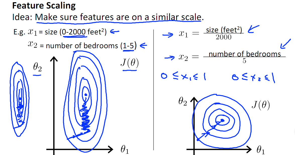
4. 从上面的观察中我们可以发现各个不同的数据的量级存在着差异,所以在后面的线性模型以及神经网络模型中我们应该先考虑进行数据的归一化或者标准化
原因:
在线性模型中多运用梯度来寻找最佳的下降方向,而树模型中则只是运用到特征的某个属性的一个特定的值来进行切分,与梯度无关。神经网络模型也是一样需要计算梯度来进行前向传递与后向反馈
进行数据的标准化处理可以提高模型的收敛速度(以下图片来自于吴恩达老师的机器学习课件)
避免给梯度数值的更新带来数值问题
有利于学习率数值的调整(因为在每个方向上的同个步长所产生的跨度是一样的)
1.2 显示数据的特征以及不重复元素的个数信息以便后续的数据处理
test_data_info = pd.DataFrame()
test_data_info['col'] = test_data.columns
unique_size = []
fea_type = []
for i in test_data.columns:
    unique_size.append(len(test_data[i].unique()))
    fea_type.append(test_data[i].dtype)
test_data_info['unique_num'] = np.array(unique_size)
test_data_info['fea_type'] = np.array(fea_type)
test_data_info
从上面的表格中我们可以得出:
Date、Operator、Failure这三个特征是字符串类型的,所以后续的处理应该考虑处理成数值类型,(因为类别比较少同时非一对多的关系)
Date.year、Date.minute、Date.second中的值都是重复的,所以没有任何意义,因此应当考虑删除
1.2.1 对非数值类型的变量进行转化
test_data.Date.unique()
test_data.Failure.unique()
test_data.Operator.unique()
对Failure与Operator进行数值的映射
test_data.Failure = test_data.Failure.apply(lambda x: 0  if x == 'No' else 1)
Operator2id = dict(zip(sorted(list(set(test_data.Operator))), range(1, len(sorted(list(set(test_data.Operator))))+1)))
test_data.Operator = test_data.Operator.apply(lambda x: Operator2id[x])
丢弃不需要的特征
test_data.drop(columns=['Date', 'Date.year', 'Date.minute', 'Date.second'], inplace=True)
将Failure转移到最后一列
temp = test_data.Failure
test_data.drop(columns=['Failure'], inplace=True)
test_data['Failure'] = temp
test_data.to_csv('./input/After_preprocessing.csv', index=False)
test_data.head()
test_data_info = pd.DataFrame()
test_data_info['col'] = test_data.columns
unique_size = []
fea_type = []
for i in test_data.columns:
    unique_size.append(len(test_data[i].unique()))
    fea_type.append(test_data[i].dtype)
test_data_info['unique_num'] = np.array(unique_size)
test_data_info['fea_type'] = np.array(fea_type)
test_data_info
2. 数据特征显示阶段
import seaborn as sns
2.1 查看failure占比,也就是正负样本的占比
plt.figure(figsize=(8, 6))
sns.countplot(test_data.Failure)

test_data.Failure.value_counts()
从上面的正负样本的比例中我们可以观察看到正负样本的比例严重失调,达到了100:1的数量级,这在后面是一定要进行处理的
- 如果不进行处理,我们可以知道在99%的情况下机器都是运行良好的,那么如果全部都猜运行良好,那么准确率的值也有99%以上,所以后面要对数据的样本比例进行调整,同时也需要对评估函数进行修正。
2.2 绘制在Failure为0与1情况下每个特征的直方图
def plot_feature_distribution(df1, df2, label1, label2, features):
    i = 0
    sns.set_style('whitegrid')
    plt.figure()
    fig, ax = plt.subplots(4,6,figsize=(24,14))

    for feature in features:
        i += 1
        plt.subplot(4,6,i)
        sns.distplot(df1[feature], hist=False, label=label1)
        sns.distplot(df2[feature], hist=False, label=label2)
        plt.xlabel(feature, fontsize=9)
        locs, labels = plt.xticks()
        plt.tick_params(axis='x', which='major', labelsize=6, pad=-6)
        plt.tick_params(axis='y', which='major', labelsize=6)
    plt.show();
t0 = test_data.loc[test_data['Failure'] == 0]
t1 = test_data.loc[test_data['Failure'] == 1]
features = test_data.columns.values[:-1]
plot_feature_distribution(t0, t1, '0', '1', features)

1. 由于正样本的比例比较少,也就是为1的时候比较少,所以会造成曲线的变化比较多,所以我们要进行观察的只需要看曲线的峰值以及大概的变化趋势是否一致
2. 可以观察得到Temperature、Humidity、Hours Since Previous Failure对于Failure的取值有着很大的关系
3. 模型构建
from sklearn.feature_selection import SelectFromModel, VarianceThreshold, SelectKBest, chi2, mutual_info_classif, f_classif
from sklearn.preprocessing import Imputer
from sklearn.ensemble import ExtraTreesClassifier
from sklearn.model_selection import train_test_split
from sklearn.metrics import roc_auc_score, accuracy_score, f1_score
from sklearn.model_selection import StratifiedKFold
from imblearn.over_sampling import SMOTE
estimate = pd.DataFrame(index=['f1_score', 'accuracy'])
X, X_test, y, y_test = train_test_split(test_data[test_data.columns[:-1]],test_data.Failure,test_size=0.3)
样本分布不均匀,使用SMOTE进行过采样
SMOTE的原理是:
- 随机选择少类中的一个样本a

然后从距离该样本较近的n的该类的样本中随机选择一个样本b
将a与b连接起来,中间的连线上随机选取一点即可作为新的该类的样本

# 对训练集进行SMOTE变换
sm = SMOTE(random_state = 42, n_jobs = -1)
X, y = sm.fit_sample(X,y)
# 划分训练集与验证集
skf = StratifiedKFold(n_splits=3, shuffle=True)
# 自定义一个metrics函数用与后面的LGBM的使用
def f1_eval(preds, train_data):
    temp = preds
    for i in range(len(temp)):
        if temp[i] >= 0.5:
            temp[i] = 1
        else:
            temp[i] = 0
    return 'f1_score', f1_score(train_data.get_label(), temp), True
# 数据的标准化处理
from sklearn.preprocessing import MinMaxScaler
standard = MinMaxScaler()
standard.fit(X)
X_standard = standard.transform(X)
X_test_standard = standard.transform(X_test)
下面都采用F1_score以及准确率评估函数进行模型的评估
- F1_score
TP(True Positive):预测答案正确
FP(False Positive):错将其他类预测为本类
FN(False Negative):本类标签预测为其他类标
其中精准度的概念如下
召回率
3.2 使用逻辑回归
from sklearn.linear_model import LogisticRegression
# 使用lbfgs的模型,也就是二阶梯度以及使用预处理之后的数据
lr = LogisticRegression(solver='lbfgs')
lr.fit(X_standard, y)
lr.score(X_test_standard, y_test)
lr_result = lr.predict(X_test_standard)
lr_result_data = pd.DataFrame(data=lr_result, columns=['lr_result'])
lr_result_data['true'] = y_test.values
estimate['logistic regression'] = np.array([f1_score(lr.predict(X_test_standard), y_test), accuracy_score(lr.predict(X_test_standard), y_test)])
print('f1_score:', f1_score(lr.predict(X_test_standard), y_test))
print('accuracy:', accuracy_score(lr.predict(X_test_standard), y_test))
lr_result_data.lr_result.value_counts()
lr_result_data.true.value_counts()
lr_result_data[lr_result_data['true'] == 1]
3.3 使用随机森林(Bagging模型)
Bagging:一个有放回采样的方式
1.对于训练数据:先进行放回采样(有些样本可能多次抽取,有些样本可能一次都没有抽取到),这个过程进行K次抽取,就得到了k个训练集。(很多机器学习模型最后的效果是因为噪声影响,在大量重复采样的过程中,我们每次采到噪声的可能性很小,我们就能更真实的看到原始数据的分布,而忽略了噪声的影响)
2.把k个训练数据进行训练,得到k个模型,最后由这k个模型进行投票得到结果。(每个模型的权重都是一样的)
from sklearn.ensemble import RandomForestClassifier
模型使用的是50个决策树以及特征抽取的方式使用sqrt的方法,树的深度最大为10
rf_valid_result = np.zeros((X.shape[0], skf.n_splits))
sub_preds = np.zeros((X_test.shape[0], skf.n_splits))
for n_fold, (train_index, vali_index) in enumerate(skf.split(X, y), start=1):
    print('fold:', n_fold)
    x_train, y_train, x_vali, y_vali = np.array(X)[train_index], np.array(y)[train_index], np.array(X)[vali_index], np.array(y)[vali_index]
    rf = RandomForestClassifier(n_estimators=50, max_features='sqrt', max_depth=10, n_jobs=2)
    rf.fit(x_train, y_train)
    print('f1_score of valid dataset :', rf.score(x_vali, y_vali))
    rf_valid_result[:, n_fold - 1] = rf.predict(X)
    sub_preds[:, n_fold - 1] = rf.predict(X_test)
显示每个特征的重要程度
plt.figure(figsize=[30, 10])
plt.bar(features, rf.feature_importances_)

rf_result = np.mean(sub_preds, axis=1)
estimate['random forest'] = np.array([f1_score(y_test, np.round(rf_result)), accuracy_score(y_test, np.round(rf_result))])
print('f1_score of test dataset:', f1_score(y_test, np.round(rf_result)))
print('accuracy_score of test dataset:', accuracy_score(y_test, np.round(rf_result)))
rf_result_data = pd.DataFrame(data=np.round(rf_result), columns=['rf_result'])
rf_result_data['true'] = y_test.values
rf_result_data.rf_result = rf_result_data.rf_result.astype(int)
rf_result_data[rf_result_data['true'] == 1]
print(rf_result_data.rf_result.value_counts())
print(rf_result_data.true.value_counts())
3.4使用lightgbm(Boosting模型)
Boosting 模型
简单的讲就是每个数据以及分类器都具有一定的权重:
初始的分布应为等概分布,也就是训练集如果有 n个样本,每个样本的分布概率为1/ n。
每次循环后提高错误样本的分布概率,分错的样本在训练集中所占权重增大,使得下一次循环的基分类器能够集中力量对这些错误样本进行判断。
最后的强分类器是通过多个基分类器联合得到的,因此在最后联合时各个基分类器所起的作用对联合结果有很大的影响,因为不同基分类器的识别率不同,他的作用就应该不同,这里通过权值体现他的作用,因此识别率越高的基分类器权重越高,识别率越低的基分类器权重越低。
import lightgbm as lgb
以下是模型的参数
param = {
    'learning_rate': 0.05,
    'boosting_type': 'gbdt',
    'objective': 'binary',
    'metric': 'auc',
    'num_leaves': 15,
    'nthread': 2,
}
sub_preds = np.zeros((X_test.shape[0], skf.n_splits))
lgb_valid_result = np.zeros((X.shape[0], skf.n_splits))
for n_fold, (train_index, vali_index) in enumerate(skf.split(X, y), start=1):
    print( n_fold)
    x_train, y_train, x_vali, y_vali = np.array(X)[train_index], np.array(y)[train_index], np.array(X)[vali_index], np.array(y)[vali_index]
    train = lgb.Dataset(x_train, label=y_train)
    vali =lgb.Dataset(x_vali, label=y_vali)
    print("training start...")
    model = lgb.train(param, train, num_boost_round=1000, valid_sets=[train, vali], early_stopping_rounds=20, verbose_eval=10, feval=f1_eval)
    lgb_valid_result[:, n_fold - 1] = model.predict(X, num_iteration=model.best_iteration)
    sub_preds[:, n_fold - 1] = model.predict(X_test,num_iteration=model.best_iteration)
plt.figure(figsize=[30, 10])
plt.bar(features, model.feature_importance(importance_type='split'))

lgb_result = np.mean(sub_preds, axis=1)
estimate['lightgbm'] = np.array([f1_score(y_test, np.round(lgb_result)), accuracy_score(y_test, np.round(lgb_result))])
print('f1 score:', f1_score(y_test, np.round(lgb_result)))
print('accuracy:', accuracy_score(y_test, np.round(lgb_result)))
lgb_result_data = pd.DataFrame(data=np.round(lgb_result), columns=['lgb_result'])
lgb_result_data.lgb_result = lgb_result_data.lgb_result.astype(int)
lgb_result_data['true'] = y_test.values
lgb_result_data[lgb_result_data['true'] == 1]
print(lgb_result_data.lgb_result.value_counts())
print(lgb_result_data.true.value_counts())
3.5 构建全连接神经网络模型
使用标准化之后的数据集
import torch
import torch.nn.functional as f
from torch.autograd import Variable
import matplotlib.pyplot as plt
# 训练集
x0 = torch.FloatTensor(X_standard)
y0 = torch.LongTensor(y)
# 测试集
x1 = torch.FloatTensor(X_test_standard)
y1 = torch.LongTensor(y_test.values)
x_, y_ = Variable(x0), Variable(y0)
网络结构如下:全连接神经网络

class Net(torch.nn.Module):
    def __init__(self, n_feature, n_hidden, n_output):
        super(Net, self).__init__()
        self.hidden = torch.nn.Linear(n_feature, n_hidden)
        self.out = torch.nn.Linear(n_hidden, n_output)

    def forward(self, x):
        x = f.relu(self.hidden(x))
        y = self.out(x)
        return y

net = Net(n_feature=23, n_hidden=100, n_output=2)
net.eval()
optimizer = torch.optim.SGD(net.parameters(), lr=0.02)
loss_func = torch.nn.CrossEntropyLoss()
for i in range(4000):
    out = net(x_)
    loss = loss_func(out, y_)
    if i % 200 == 0:
        print(loss)
    optimizer.zero_grad()
    loss.backward()
    optimizer.step()
X_predicteds = []
_, predicted = torch.max(net(x_), 1)
X_predicteds.extend(predicted.int().tolist())
predicteds = []
_, predicted = torch.max(net(x1), 1)
predicteds.extend(predicted.int().tolist())
estimate['dnn'] = np.array([f1_score(np.array(predicteds) ,y_test.values), accuracy_score(np.array(predicteds) ,y_test.values)])
print('f1_score', f1_score(np.array(predicteds) ,y_test.values))
print('accuracy_score', accuracy_score(np.array(predicteds) ,y_test.values))
dnn_result_data = pd.DataFrame(data=np.array(predicteds), columns=['dnn_result'])
dnn_result_data['true'] = y_test.values
dnn_result_data[dnn_result_data['true'] == 1]
print(dnn_result_data.dnn_result.value_counts())
print(dnn_result_data.true.value_counts())
3.6 使用stacking进行模型融合

使用的方法是将上面四种模型的结果进行结合,然后使用随机森林再进行第二层分类
rf_valid = np.mean(rf_valid_result, axis=1)
lgb_valid = np.mean(lgb_valid_result, axis=1)
new_X = pd.DataFrame()
new_X['lr'] = lr.predict(X_standard)
new_X['rf'] = rf_valid
new_X['lgb'] = lgb_valid
new_X['dnn'] = np.array(X_predicteds)
new_X_test = pd.DataFrame()
new_X_test['lr'] = lr.predict(X_test_standard)
new_X_test['rf'] = rf_result
new_X_test['lgb'] = lgb_result
new_X_test['dnn'] = np.array(predicteds)
sub_preds = np.zeros((new_X_test.shape[0], skf.n_splits))
for n_fold, (train_index, vali_index) in enumerate(skf.split(new_X, y), start=1):
    print( n_fold)
    x_train, y_train, x_vali, y_vali = np.array(new_X)[train_index], np.array(y)[train_index], np.array(new_X)[vali_index], np.array(y)[vali_index]
    rf = RandomForestClassifier(n_estimators=10, max_features=2, max_depth=2, n_jobs=2)
    rf.fit(x_train, y_train)
    print(rf.score(x_vali, y_vali))
    sub_preds[:, n_fold - 1] = rf.predict(new_X_test)
stacking_result = np.mean(sub_preds, axis=1)
estimate['stacking'] = np.array([f1_score(y_test, np.round(stacking_result)), accuracy_score(y_test, np.round(stacking_result))])
print('f1_score:', f1_score(y_test, np.round(stacking_result)))
print('accuracy:', accuracy_score(y_test, np.round(stacking_result)))
stacking_result_data = pd.DataFrame(data=np.round(stacking_result), columns=['stacking_result'])
stacking_result_data['true'] = y_test.values
stacking_result_data.stacking_result = stacking_result_data.stacking_result.astype(int)
stacking_result_data[stacking_result_data['true'] == 1]
print(stacking_result_data.stacking_result.value_counts())
print(stacking_result_data.true.value_counts())
estimate
result_data = pd.DataFrame(data=np.round(lr_result), columns=['lr_result'])
result_data['rf_result'] = np.round(rf_result)
result_data['lgb_result'] = np.round(lgb_result)
result_data['dnn_result'] = np.array(predicteds)
result_data['stacking_result'] = np.round(stacking_result)
result_data['true'] = y_test.values
result_data.lr_result = result_data.lr_result.astype(int)
result_data.rf_result = result_data.rf_result.astype(int)
result_data.stacking_result = result_data.stacking_result.astype(int)
result_data.lgb_result = result_data.lgb_result.astype(int)
result_data[dnn_result_data['true'] == 1]
4. 总结
从这一次项目中自己最有体会以及学习最多的就是类别分布不均匀的状况,一开始没有注意到这个问题,然后用随机森林跑出来的结果用准确率评估之后达到了99%,不过自己刚好想看看什么时候出现了故障的情况,结果发现了没有存在预测值为1的情况,于是寻找问题,最终发现了正负比例高达1:100,于是得思考对于非平衡的数据集该如何进行处理,经过查阅网上的资料,知道了过采样与欠采样的方法,于是使用了过采样的方法之后虽然模型的准确度下降,但是预测为正样本正确的情况达到了70%左右
之前自己比较擅长的是线性模型以及树模型,而在这一次的项目中自己第一次使用了神经网络,虽然很简陋,但是使用非常方便和快捷。不过可能是因为模型或者参数的问题,神经网络的结果没有十分得乐观。
第一次尝试了模型融合,使用stacking的方法将前面4中模型进行融合,并且得到了更好的结果,这让我感到很兴奋,不过因为自己写得模型并没有很多,所以后面应该尝试更多的模型的融合。
感谢老师与师姐的教导,这一次项目使自己学习颇丰,谢谢!